Quantum simulation for material science, chemistry and physics
This scenario describes the how quantum computing can be used for material science, chemistry and physics.
It has the following specification:
- Input: molecule specification
- Output: ground state energy
- Used in:
- material science
- battery design
- catalyst research
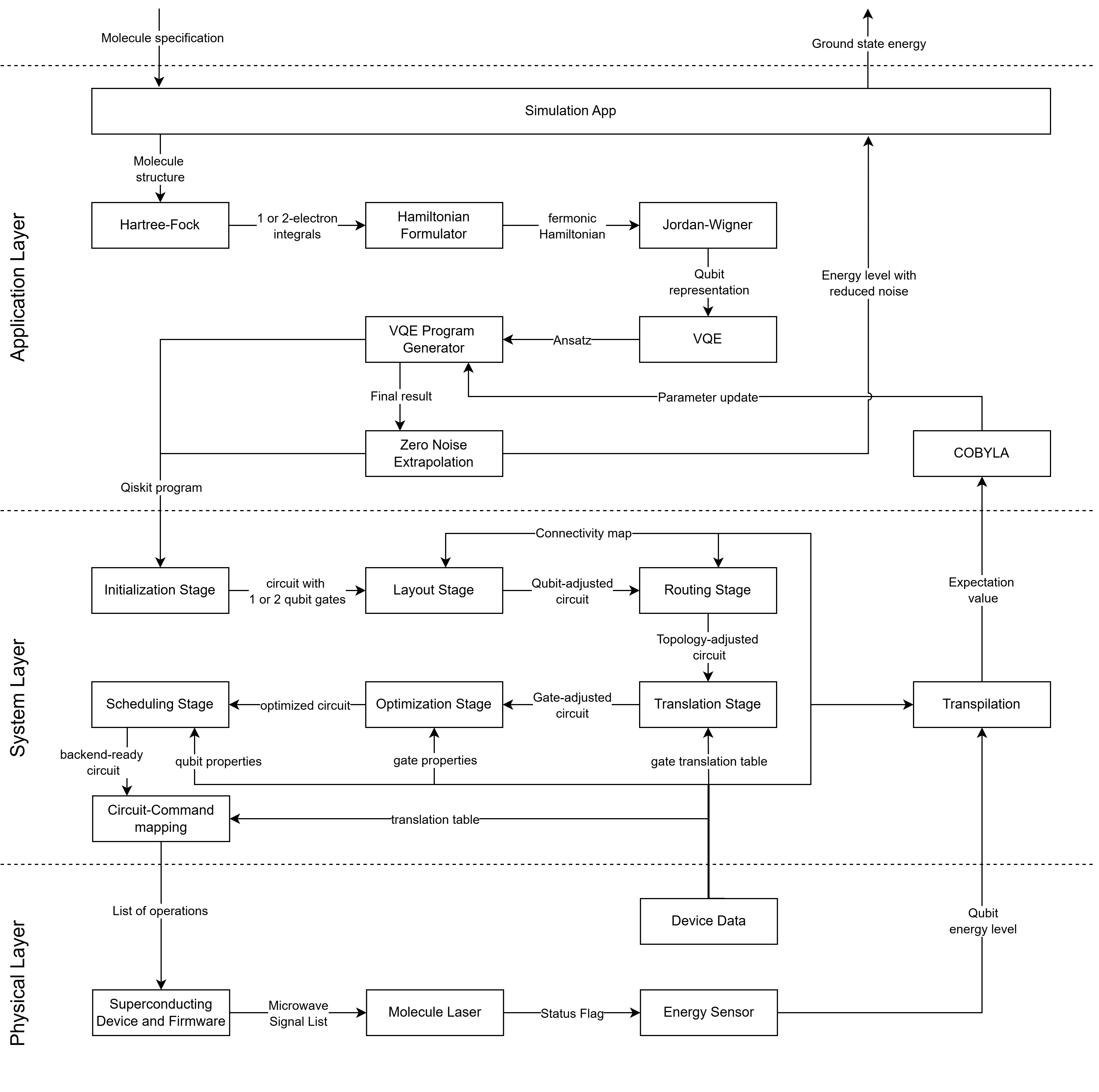
Application Layer - Downwards
-
Simulation App:
- The Simulation App is the entry point for this scenario.
- It takes the molecule specification and passes it down to the Hartree-Fock algorithm
-
Hartree-Fock:
- The Hartree-Fock algorithm is the first transformation step to get from the molecule input to a quantum ready representation
- Its input is the molecular geometry in our scenario
- The output are the electron integrals.
-
Hamiltonian Formulator:
- The Hamiltonian formulation maps the electron integrals into a fermonic Hamiltonian.
-
Jordan-Wigner:
- The Jordan-Wigner Transformation allows a qubit representation using a fermonic Hamiltonian and turns it into a spin Hamiltonian, which is equivalent to a set of qubits.
-
VQE (Variational Quantum Eigensolver):
- The VQE Algorithm is a hybrid algorithm, which uses the qubit Hamiltonian to create a parameterised quantum circuit.
-
VQE Program Generator
- With the parametrised circuit the program generator creates a program for the transpilation pipeline in the system layer.
System Layer - Downwards
The Qiskit Transpilation Pipeline consists of 6 steps:
-
Initialization Stage
- Using the quantum program from the Application Layer, the transpilation pipeline can start.
- The first step of the transpilation pipeline is breaking down multi- and custom made qubit- gates into one- or two-qubit operations.
-
Layout Stage
- This stage maps the input circuit's virtual qubits to the target's physical hardware qubits.
- The algorithm's goal is to map the qubits in such a way that frequently-interacting virtual qubits end up next to each other in the physical hardware.
-
Routing Stage
- As described in the step before, a perfect connectivity between the qubits can not always be achieved. Therefore this stage adds additional operations to adapt to these constraints.
- Using the circuit and hardware topology as inputs, it can create a physically compatible circuit by inserting SWAP gates to move information between previously disconnected qubits.
-
Translation Stage
- This stage rewrites all previously chosen gates into the specific native gates supported by the target hardware's Instruction Set Architecture (ISA).
-
Optimization Stage
- This stage executes low-level, hardware-aware refinements on circuits that are already compatible with the target's Instruction Set Architecture (ISA) to reduce redundancy.
-
Scheduling Stage
- The scheduling stage receives an ISA-compatible circuit and inserts explicit delay instructions to accurately reflect qubit idle periods, hardware timing constraints and to reduce error rate.
- It ensures the final output remains ISA-compatible while updating start-time metadata and optionally applying walltime-sensitive transformations.
- This concludes the Qiskit transpilation pipeline.
-
Circuit-Command Mapping
- Using the ISA-compatible circuit, additional information like number of measurements demanded and a translation table, which translated the commands into backend compatible commands, this steps gives a list of operations to the device and firmware of the hardware.
Physical Layer
-
Superconducting Device and Firmware:
- Using digital hardware instructions and pulse definitions, this process converts these commands into physical signals to control operations on the quantum chip.
- It outputs a microwave signal list directly to the quantum hardware, translating digital instructions into executable physical actions.
-
Molecule Laser:
- The molecule laser uses the microwave signal list to execute the quantum operations on the physical hardware.
- When all operations are done, the molecule Laser sends a status flag to the energy sensor
-
Energy Sensor:
- When the molecule laser has completed its job and updated its status, this step measures the qubit energy levels
System Layer - Upwards
- Transpilation
- In this step, the qubit energy levels are transformed into an expectation value.
- To do this, additional backend data is needed to interpret the measured results.
Application Layer - Upwards
-
COBYLA
- COBYLA is a classical optimizer which needs an expectation value as input.
- It compares the expectation value to the last one (if it exists) and tries to optimize the parameters of the VQE algorithm.
- After an local optimal solution is found or the maximum of iterations is reached, the classical optimizer terminates
-
VQE Program Generator
- The Program Generator updates the parameters of the COBYLA algorithm and starts the process again.
- When the classical optimizer terminates, the Program Generator gives the optimal result towards the Error Mitigation Method.
-
Zero Noise Extrapolation
- Zero Noise Extrapolation (ZNE) is a error mitigation method, which can reduce the error rate by using an expectation value and a circuit has input
- It creates a program to measure a new expectation value with a circuit, which has still the same function but uses more gates.
- This process is repeated multiple times and lead towards a noise pattern, which allows to reduce the error rate by extrapolation.
-
Simulation App
- The error-optimized expectation value is given towards the simulation app, which then visualize it as ground state energy for the user.